Code and Output
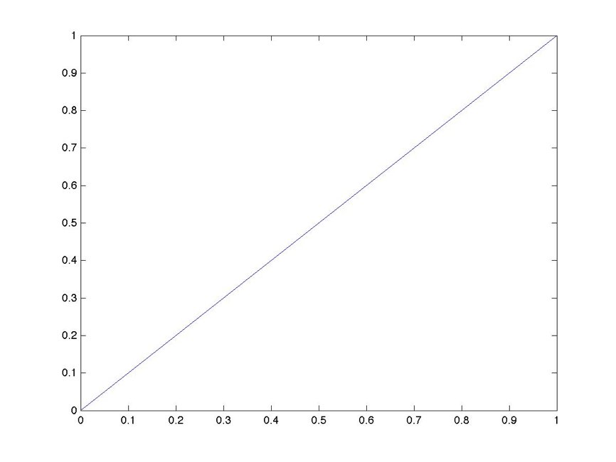
Code 10.1.1:
clear all
close all

figure(1)
x = [0 1];
y = [0 1];
box on
our_first_line = plot(x, y);
Output 10.1.1:
Code 10.1.2:
get(our_first_line)
Output 10.1.2:
Color = [0 0 1]
EraseMode = normal
LineStyle = -
LineWidth = [0.5]
Marker = none
MarkerSize = [6]
MarkerEdgeColor = auto
MarkerFaceColor = none
XData = [0 1]
YData = [0 1]
ZData = []

BeingDeleted = off
ButtonDownFcn =
Children = []
Clipping = on
CreateFcn =
DeleteFcn =
BusyAction = queue
HandleVisibility = on
HitTest = on
Interruptible = on
Parent = [151.008]
Selected = off
SelectionHighlight = on
Tag =
Type = line
UIContextMenu = []
UserData = []
Visible = on
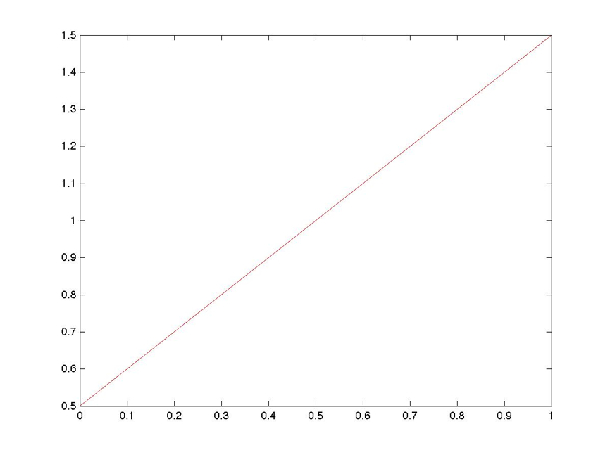
Code 10.1.3:
figure(2)
delta_y = .5;
our_second_line = plot([min(x)  max(x)],...
           [min(y)+ delta_y max(y) + delta_y],'color',[1 0 0]);
box on
Output 10.1.3:
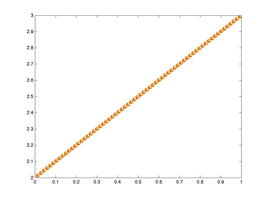
Code 10.1.4:
figure(3)
delta_y = 1;
our_third_line = plot([min(x)  max(x)],...
   [min(y)+ 2*delta_y max(y) + 2*delta_y]);
set(our_third_line,'color',[.9 .5 .1], ...
    'linestyle','--', ...
    'linewidth',8);
box on
Output 10.1.4:
Code 10.1.5:
set(gca,'XGrid')
set(gcf,'PaperOrientation')
Output 10.1.5:
[ on | {off} ]
[ {portrait} | landscape | rotated ]
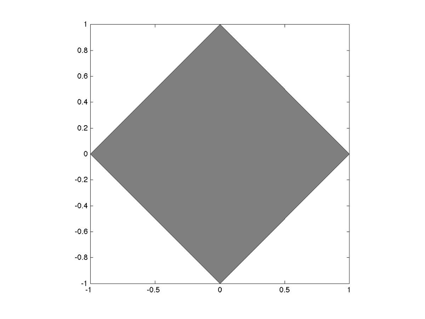
Code 10.2.1:
function my_polygon_1(n,r,c)

x = linspace(0,2*pi,n+1)
x = r*cos(x)

y = linspace(0,2*pi,n+1)
y = r*sin(y);

fill(x,y,c)
Code 10.2.2:
figure(4)
my_polygon_1(4,1,[.5 .5 .5])
axis square
Output 10.2.2:
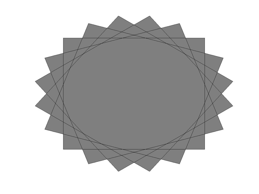
Code 10.2.3:
function my_polygon_2(n,r,c,turn)

x = linspace(0,2*pi,n+1)
x = x + (turn + 1/(2*n))*(2*pi);
x = r*cos(x);

y = linspace(0,2*pi,n+1)
y = y + (turn + 1/(2*n))*(2*pi);
y = r*sin(y);

fill(x,y,c)
Code 10.2.4:
figure(5)
hold on
for turn = linspace(-.2,0,5)
    my_polygon_2(4,1,[.5 .5 .5],turn)
    axis off
end
Output 10.2.4:
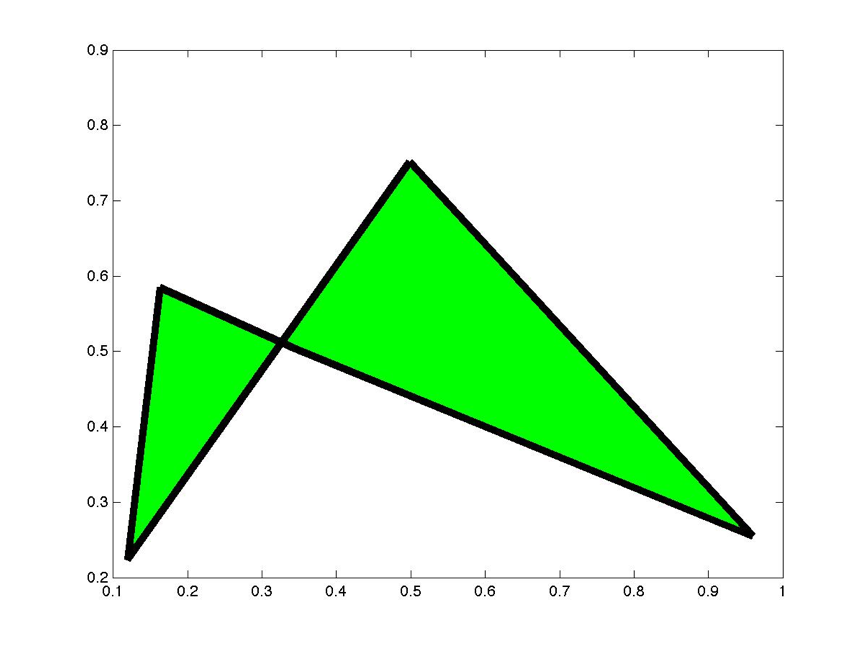
Code 10.2.5:
figure(6)
crazy_x = rand(1,5);
crazy_y = rand(1,5);
f = fill(crazy_x,crazy_y,'g')
set(f,'LineWidth', 5.0);
Output 10.2.5:
10.3 Loading Images
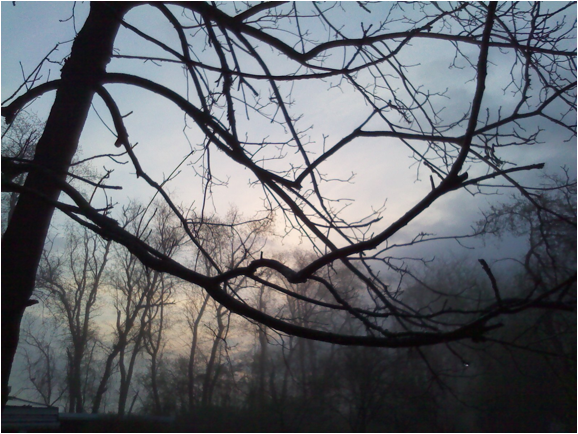
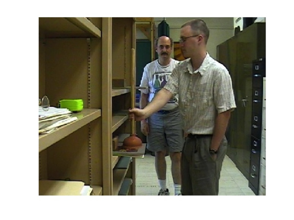
Code 10.3.1:
figure(8)
a = imread('view_from_window.jpg');
image(a)
axis off
Output 10.3.1:
Code 10.3.2:
figure(9)
b = imread('lab_photo.jpg');
image(b)
axis off
Output 10.3.2:
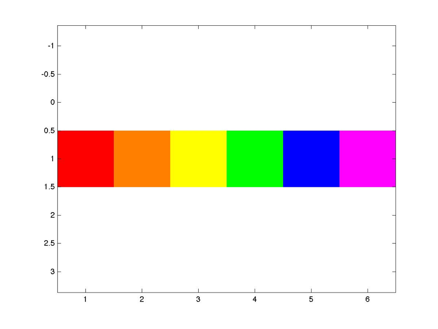
Code 10.4.1:
clf;
clear;
Rainbow(1,1:6,1:3) = [
    1 0 0   % Red
    1 .5 0  % Orange
    1 1 0   % Yellow
    0 1 0   % Green
    0 0 1   % Blue
    1 0 1   % Violet
    ];
image(Rainbow)
axis equal
Output 10.4.1:
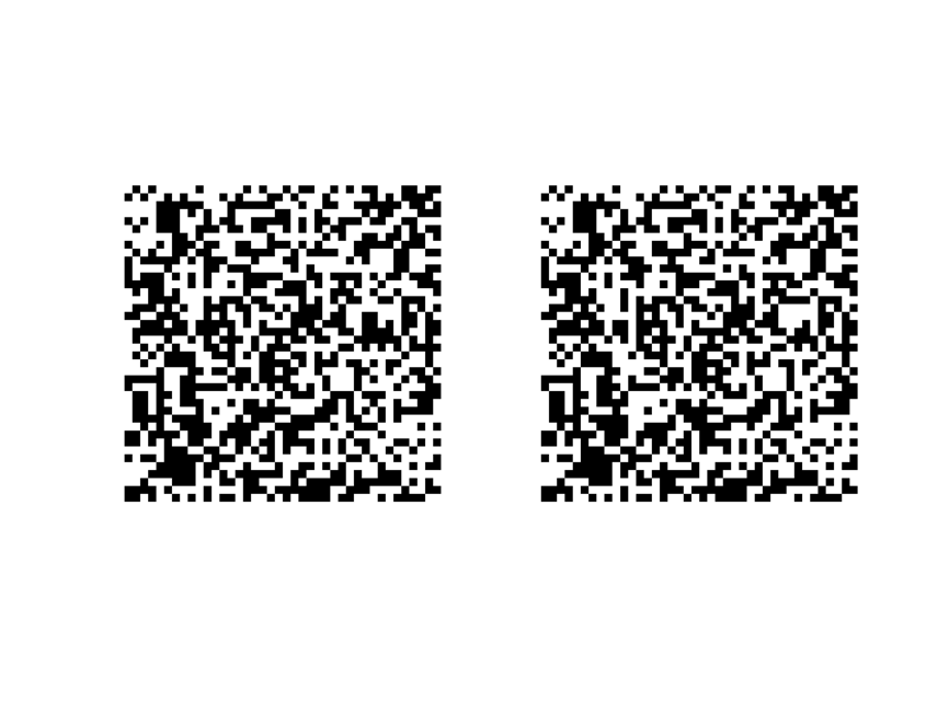
Code 10.4.2:
% Set up
figure(10)
windowposition = [10,550,1000 500];
set(10,'Position',windowposition);
% Make Identical Images
RightEyePicture = randi(2,40,40);
LeftEyePicture = RightEyePicture;
% Shift and superimpose an inner square
InnerSquare = randi(2,20,20);
RightEyePicture(11:30,11:30) = InnerSquare;
LeftEyePicture(11:30,13:32) = InnerSquare;
% Define color map, row 1 = white, row 2 = black
mycolors = [
     1 1 1
     0 0 0
     ];
colormap(mycolors);
% Display
subplot(1,2,1);
image(RightEyePicture);
title('Right','fontsize',16)
axis off;
axis equal
subplot(1,2,2);
image(LeftEyePicture);
title('Left','fontsize',16)
axis off;
axis equal
shg
Output 10.4.2:
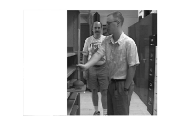
Code 10.5.1:
b = imread('lab_photo.jpg');
image(b);
hold on;
[x y] = ginput(2);
xs = [x(1) x(2) x(2) x(1)];
ys = [y(1) y(1) y(2) y(2)];
fill(xs,ys,'w');
Output 10.5.1:
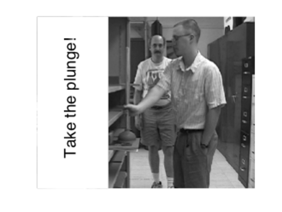
Code 10.5.2:
clear x y
[x y] = ginput(1);
text(x,y,'Take the plunge!','rotation',90,'fontsize',24);
Output 10.5.2:
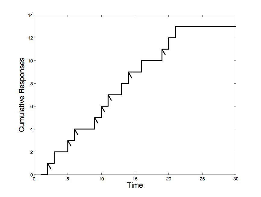
Code 10.6.1:
responses(1) = 0;
responses(2:21) = randi(2,1,20)-1;
    responses(22:30) = 0;
cumrec = cumsum(responses);
reinforcedtrials = [];
for i = 1:20
    if responses(i) > 0 && randi(2) > 1
        reinforcedtrials = [reinforcedtrials i];
    end
end
stairs(cumsum(responses));
hold on
for i = 1:length(reinforcedtrials)
    j = reinforcedtrials(i);
    plot([j j+.5], [cumrec(j) cumrec(j)-.5]);
end
xlabel('Time','Fontsize',16);
ylabel('Cumulative Responses','Fontsize',16);
Output 10.6.1:
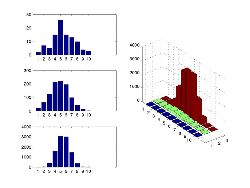
Code 10.7.1:
m = [];
for j = 2:4
    clear n x
    [n x] = hist(randn(1,10^j),10);
    subplot(3,2,((j-1)*2)-1)
    bar(n)
    m = [m;n];
end
subplot(3,2,[2 4 6])
bar3(m')
Output 10.7.1:
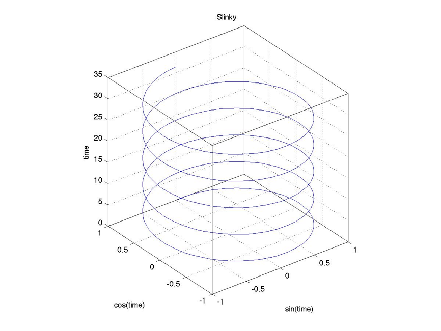
Code 10.8.1:
figure(3)
t = 0:pi/50:10*pi;
plot3(sin(t),cos(t),t)
axis square;
grid on
box on
xlabel('sin(time)','rotation',0);
ylabel('cos(time)','rotation',-0);
zlabel('time');
title('Slinky');
Output 10.8.1:
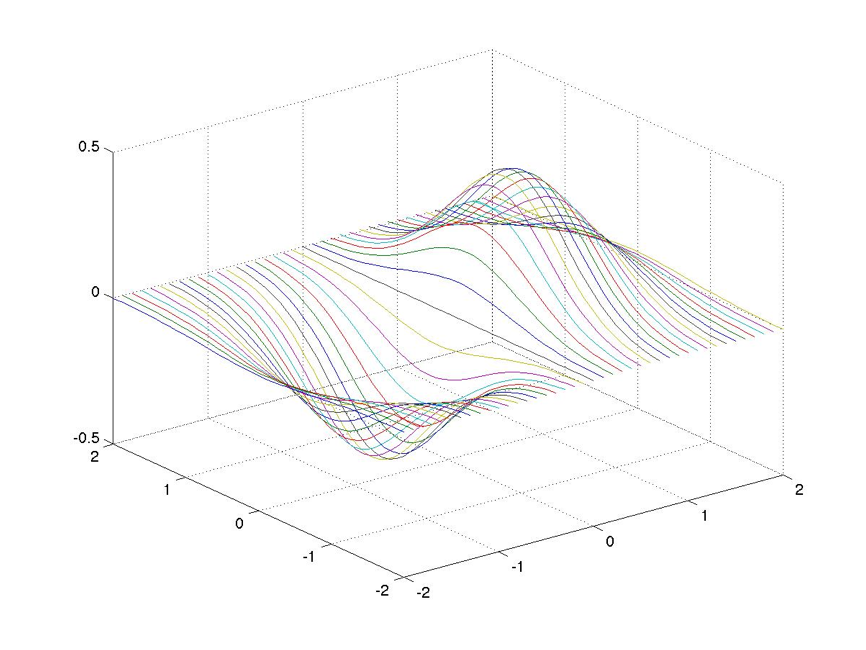
Code 10.9.1:
figure(4)
[X,Y] = meshgrid(linspace(-2,2,41));
Z = X.*exp(-X.^2 - Y.^2);
plot3(X,Y,Z)
grid on
Output 10.9.1:
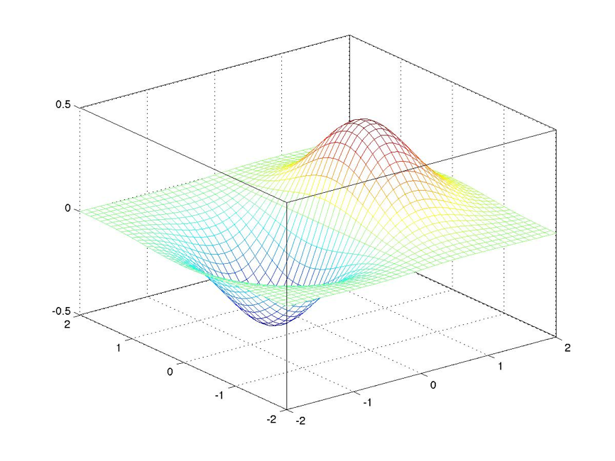
Code 10.10.1:
figure(5)
mesh(X,Y,Z)
box on
Output 10.10.1:
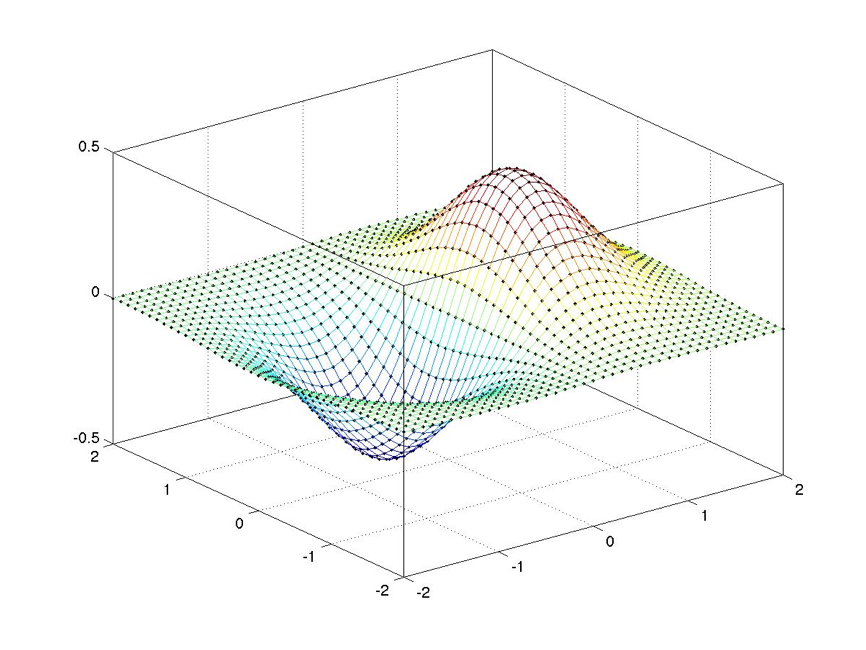
Code 10.10.2:
figure(6)
mesh(X,Y,Z)
hold on
plot3(X,Y,Z,'k.')
box on
Output 10.10.2:
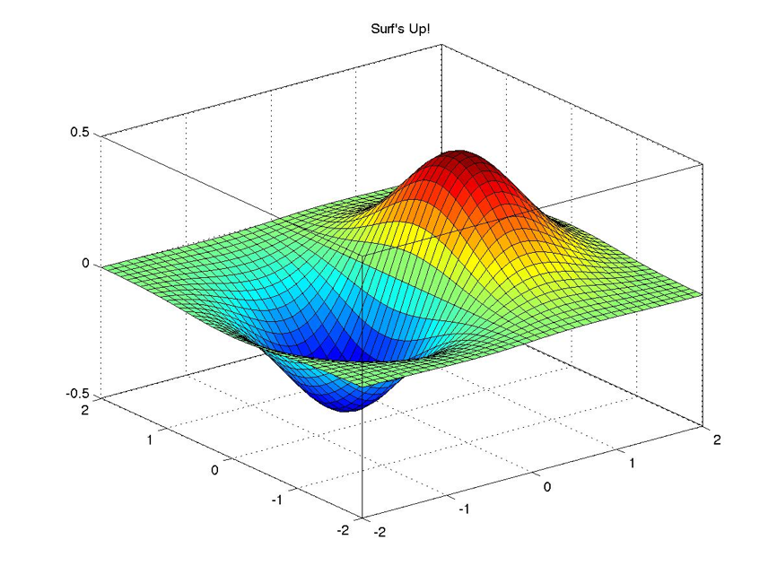
Code 10.11.1:
figure(7)
surf(X,Y,Z)
title('Surf''s Up!')
box on
Output 10.11.1:
Code 10.12.1:
help view
Output 10.12.1:
VIEW   3-D graph viewpoint specification.
VIEW(AZ,EL) and VIEW([AZ,EL]) set the angle of the view from which an
observer sees the current 3-D plot.  AZ is the azimuth or horizontal
rotation and EL is the vertical elevation (both in degrees). Azimuth
revolves about the z-axis, with positive values indicating counter-
clockwise rotation of the viewpoint. Positive values of elevation
correspond to moving above the object; negative values move below.
VIEW([X Y Z]) sets the view angle in Cartesian coordinates. The
magnitude of vector X,Y,Z is ignored.
Code 10.12.2:
figure(8)
surf(X,Y,Z)
set(gca,'view',[0,90])
Output 10.12.2:
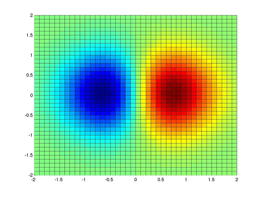
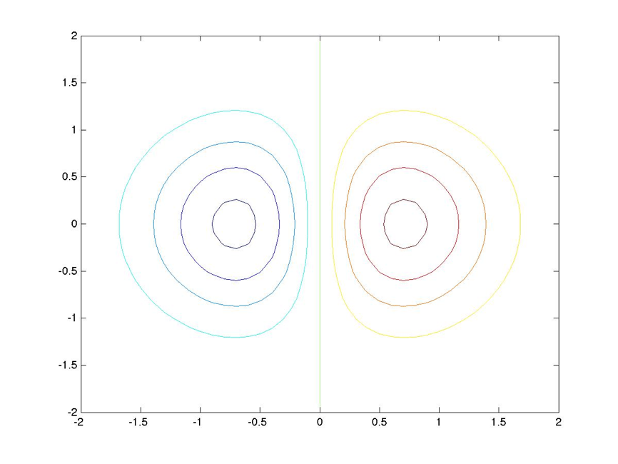
Code 10.13.1:
figure(9)
contour(X,Y,Z)
Output 10.13.1:
Code 10.14.1:
[x,y] = meshgrid(1:8)
Output 10.14.1:
x =

1   2   3   4   5   6   7   8
1   2   3   4   5   6   7   8
1   2   3   4   5   6   7   8
1   2   3   4   5   6   7   8
1   2   3   4   5   6   7   8
1   2   3   4   5   6   7   8
1   2   3   4   5   6   7   8
1   2   3   4   5   6   7   8

y =

1   1   1   1   1   1   1   1
2   2   2   2   2   2   2   2
3   3   3   3   3   3   3   3
4   4   4   4   4   4   4   4
5   5   5   5   5   5   5   5
6   6   6   6   6   6   6   6
7   7   7   7   7   7   7   7
8   8   8   8   8   8   8   8
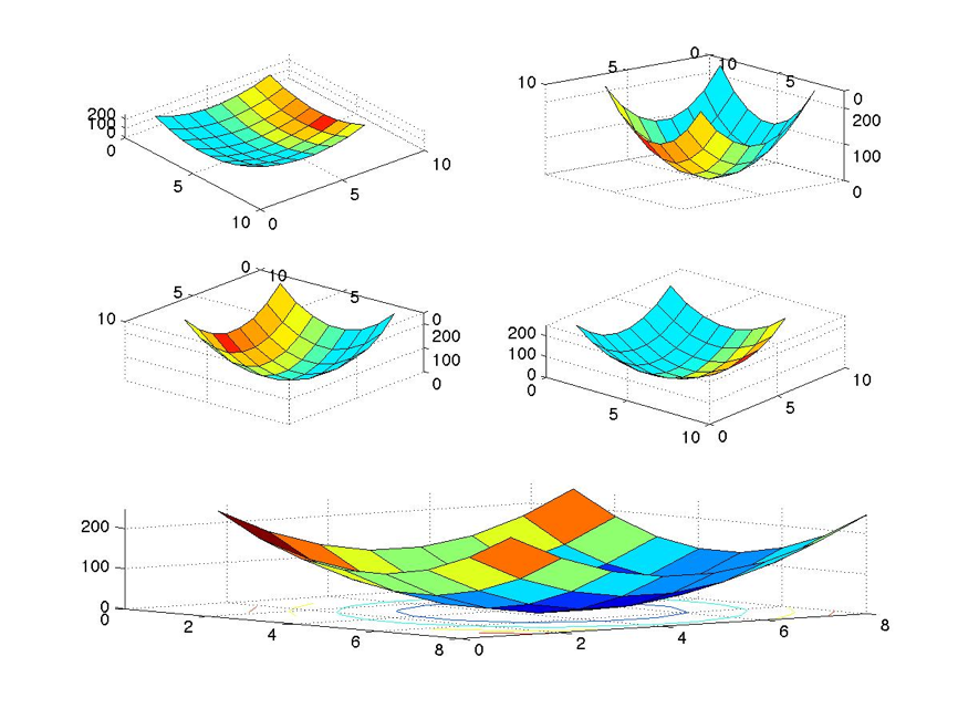
Code 10.14.2:
figure(10)
z = (10*(x-mean(mean(x))).^2) + (10*(y-mean(mean(y))).^2);

for v = 1:5
   if v < 5
     subplot(3,2,v)
     surfl(x,y,z)
   else
     subplot(3,2,5:6)
     surfc(x,y,z)
   end
   zlim([0 max(max(z))+2]);
   set(gca,'view',[50.5 v*76.2987]);
end
Output 10.14.2:
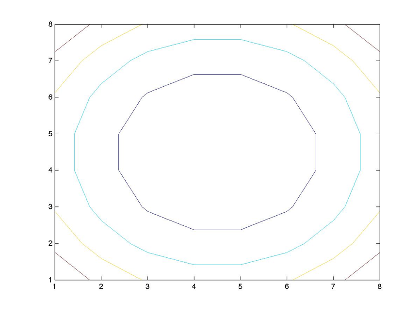
Code 10.14.3:
contour(x,y,z)
Output 10.14.3:
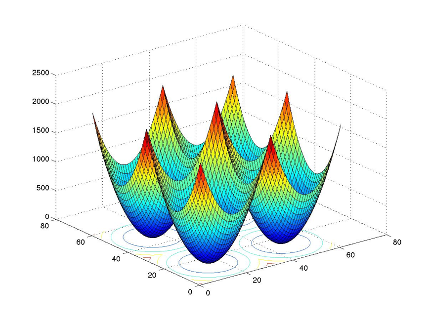
Code 10.14.4:
figure(3)
[x,y] = meshgrid(1:61);
[rows columns] = size(x);

x_low_attractor = .5*mean(mean(x));
x_high_attractor = 1.5*mean(mean(x));
y_low_attractor = .5*mean(mean(y));
y_high_attractor = 1.5*mean(mean(y));

k = 5;

for r = 1:rows
  for c = 1:columns
    if abs(x(r,c)-x_low_attractor) <= ...
       abs(x(r,c)-x_high_attractor)
      x_attractor = x_low_attractor;
    else
      x_attractor = x_high_attractor;
    end
    if abs(y(r,c)-y_low_attractor) <= ...
       abs(y(r,c)-y_high_attractor)
      y_attractor = y_low_attractor;
    else
      y_attractor = y_high_attractor;
    end
    z(r,c) = (k*(x(r,c)-x_attractor).^2) + ...
         (k*(y(r,c)-y_attractor).^2);
  end
end

surfc(x,y,z)
Output 10.14.4:
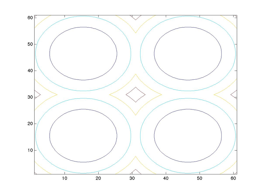
Code 10.14.5:
figure(4)
contour(x,y,z)
Output 10.14.5:
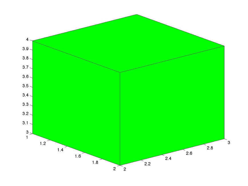
Code 10.15.1:
function drawcube=cube(coord);

% coord = 1x3 front/bottom/left coordinates matrix

x = coord(1);
y = coord(2);
z = coord(3);

vertices_matrix = [[x y z];[x+1 y z];[x+1 y+1 z];[x y+1 z]; ...
        [x y z+1];[x+1 y z+1];[x+1 y+1 z+1];[x y+1 z+1]];

faces_matrix = [[1 2 6 5];[2 3 7 6];[3 4 8 7];[4 1 5 8];...
        [1 2 3 4];[5 6 7 8]];

drawcube = patch('Vertices',vertices_matrix,'Faces',faces_matrix,...
    'FaceColor','g');
Code 10.15.2:
cube([1 2 3])
Output 10.15.2:
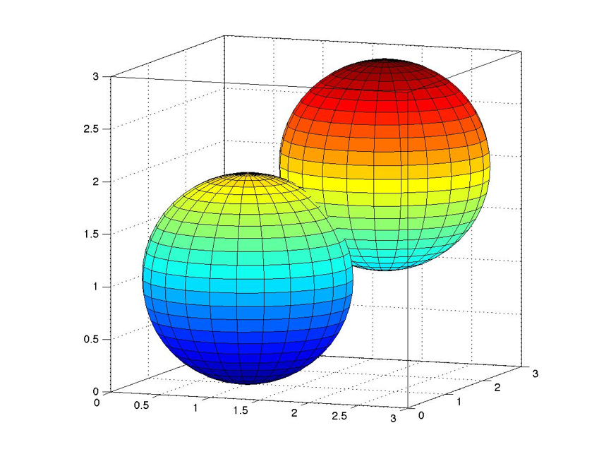
Code 10.16.1:
figure(5)
[x y z] = sphere(24);
hold on
for j = 1:2
  surf(x + j,y + j, z + j);
end
axis equal
grid on
box on
view(21,8)
Output 10.16.1:
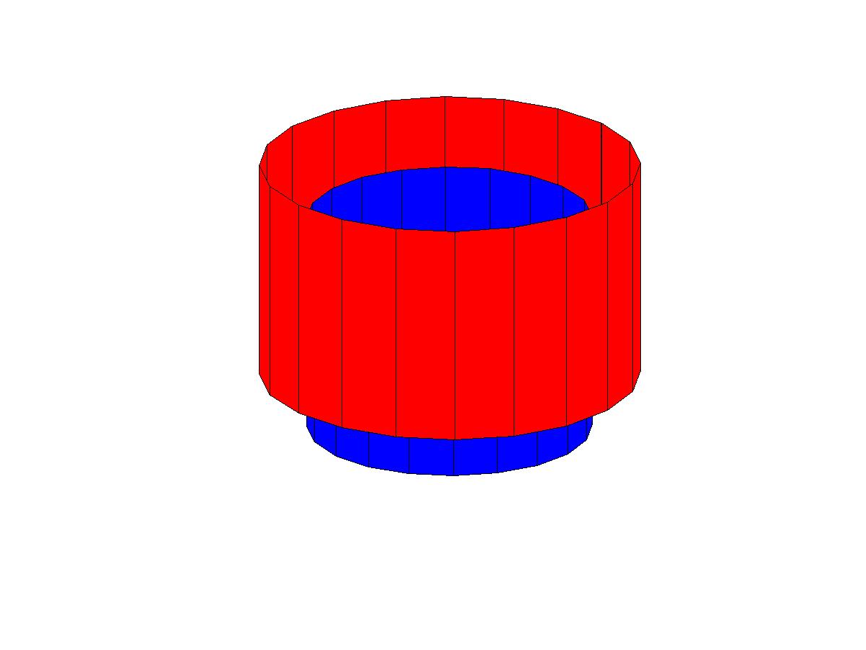
Code 10.16.2:
figure(6)
hold on
AZ = -37.5,;
EL = 30;
view(AZ,EL)
for j = 1:2
  if j == 1
    [x y z] = cylinder(24);
    k = 1;
    s = surf(x + k,y + k, z + k);
    set(s,'facecolor','r');
  else
    k = .75;
    [x y z] = cylinder(18);
    s = surf(x + k,y + k, z + k);
    set(s,'facecolor','b');
  end

end
axis off
Output 10.16.2:
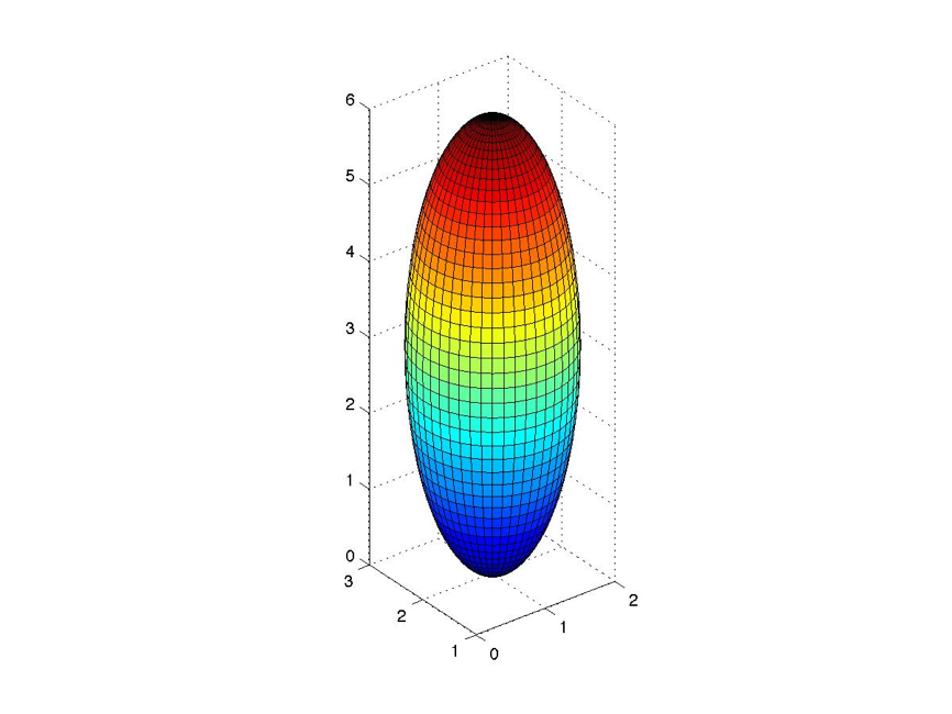
Code 10.17.1:
xc = 1; yc = 2; zc = 3;
xr = 1; yr = 1, zr = 3;
n_facets = 48;
[x,y,z]=ellipsoid(xc,yc,zc,xr,yr,zr,n_facets);
surf(x,y,z);
axis equal;
Output 10.17.1:
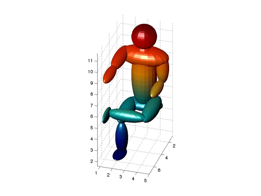
Code 10.17.2:
% Ellipsoid_Man_Matt_Walsh
% March_23_2006

close all
clear all
clc

figure(1)
%thorax
[x y z]=ellipsoid(2,3,7.3,1,1,3);
surf(x,y,z);

%head
hold on
[x y z]=ellipsoid(2,3,10.7,1,1,1);
surf(x,y,z);

%shoulder mass
[x y z]=ellipsoid(2,3,9,1,2,.8);
surf(x,y,z);

%right arm
[x y z]=ellipsoid(3.2,1.4,9.2,1.8,.5,.5);
surf(x,y,z);

%right forearm
[x y z]=ellipsoid(5.9,1.4,9.2,1.3,.4,.4);
surf(x,y,z);

%left forearm
[x y z]=ellipsoid(3.5,4.5,7.1,1.3,.4,.4);
surf(x,y,z);

%left arm
[x y z]=ellipsoid(2,4.5,8.1,.5,.5,1.3);
surf(x,y,z);

%right thigh
[x y z]=ellipsoid(3.33,4,5.1,1.9,.6,.6);
surf(x,y,z);

%left thigh
[x y z]=ellipsoid(3.33,2,4.7,1.9,.6,.6);
surf(x,y,z);

%bubble butt
[x y z]=ellipsoid(2,3,4.7,.8,1.5,.5);
surf(x,y,z);

%right calf
[x y z]=ellipsoid(4.7,2,3,.5,.5,1.4);
surf(x,y,z);

%left calf
[x y z]=ellipsoid(5,2.5,5.2,.5,1.6,.5);
surf(x,y,z);

%left foot
[x y z]=ellipsoid(5.4,1,5.2,1,.2,.505);
surf(x,y,z)

%right foot
[x y z]=ellipsoid(5.2,2,1.8,1,.505,.2);
surf(x,y,z);

grid on
axis on
zlim =[0 20];
shading interp;
light;
axis equal
set (gca,'view',[107,30], 'AmbientLightColor', [1 0 0] );
Output 10.17.2:
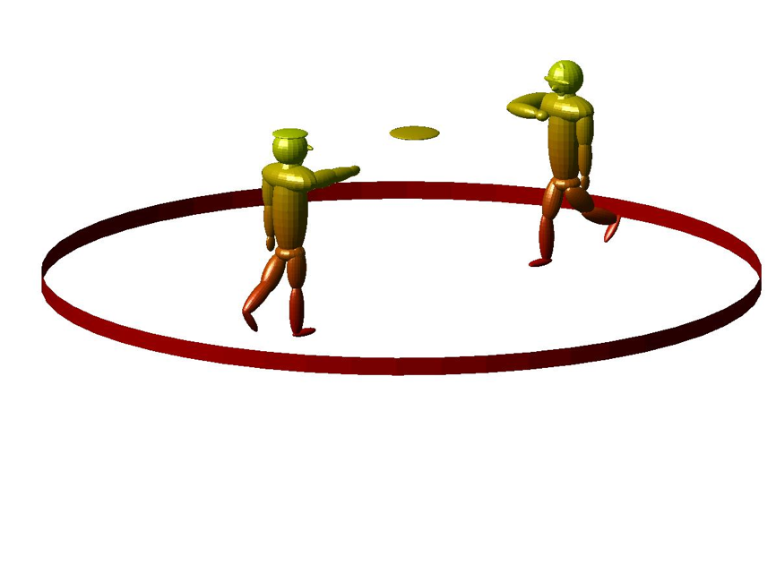
Code 10.17.3:
% Playing_frisbee_Robrecht_Van_Der_Wel.m
% March_23_2006

close all
clear all
clc

figure(1)
set(gcf, 'Color', [.2 .8 .8]);
title('Playing frisbee', 'FontSize', 20);
colormap(autumn);

subplot(4,2,[1:6]);
% Frisbee person
% Order is: Head, mouth/hair, eyes, nose, shoulders,
% torso, gluteus,  left arm, left
% forearm, left hand, right arm, right forearm,
% right hand, right calf, right foot

hold on
%Head M/H Eyes Nose Shou Tors GM LA LFA LH RA  RFA   RH  RC   RF
x_1 = [-10  -9.5 -9.2 -9.2 -10 -10 -10  -10  -10  -10 ...
    -8.8  -7.3   -7.2  -9.0 -8.5];
y_1 = [3  3.1  3.1 3.1   3  3   3  4.5  4.5  4.5  1.4 ...
     2.4   3.9  2.5   2.5];
z_1   = [10.7 10.7  10.7 10.3  9  7.3 4.7 8.1  6.5  5 ...
     9.2   9.2   9.2  1.7   .3];
x_rad_1 = [1  .2   .2 .4   1  1  .8  .5  .4  .3  1.8 ...
      .4  .35  .45   .9];
y_rad_1 = [1  .5   1  .2   2  1  .9  .5  .4  .2   .5 ...
     1.3  .4  .4   .3];
z_rad_1 = [1  1   .2 .2   .8  3  .5  1.3  1.3  .5   .5 ...
      .4  .3  1.5   .2];

for i = 1:length(x_1)
  [xpos_1 ypos_1 zpos_1]= ...
  ellipsoid(x_1(i),y_1(i),z_1(i),x_rad_1(i),y_rad_1(i),z_rad_1(i));
  surf(xpos_1,ypos_1,zpos_1);
end
shading interp;
light;

[xpos_1 ypos_1 zpos_1]=ellipsoid(-13.1,3.6,1.6,.9,.3,.2);
left_foot_1 = surf(xpos_1,ypos_1,zpos_1);
zdir = [0 1 0];
center = [-13.1,3.6,1.6];
rotate(left_foot_1,zdir,50,center);

[xpos_1 ypos_1 zpos_1]=ellipsoid(-10.5,3.6,3.75,.6,.5,1.3);
left_thigh_1 = surf(xpos_1,ypos_1,zpos_1);
zdir = [0 1 0];
center = [-10.5,3.6,3.75];
rotate(left_thigh_1,zdir,50,center);

[xpos_1 ypos_1 zpos_1]=ellipsoid(-12.1,3.6,2.5,.45,.4,1.5);
left_calf_1 = surf(xpos_1,ypos_1,zpos_1);
zdir = [0 1 0];
center = [-12.1,3.6,2.5];
rotate(left_calf_1,zdir,70,center);

[xpos_1 ypos_1 zpos_1]=ellipsoid(-9.4,2.6,3.8,.6,.5,1.3);
right_thigh_1 = surf(xpos_1,ypos_1,zpos_1);
zdir = [0 1 0];
center = [-9.4,2.6,3.8];
rotate(right_thigh_1,zdir,160,center);

% Catching person
% Order is: Head, hat,mouth/hair, eyes, nose, shoulders,
% torso, gluteus, left arm,
% left forearm, left hand, right arm, right forearm, right hand,
% right thigh,right calf, right foot
hold on
x_2 = [12 12 11.5 11.3 11.3 12 12 12 12 12 12 11 9.8 8.5 12 ...
  12 11.4];
y_2 = [3 3 3.1 3.1 3.1 3 3 3 1.5 1.5 1.5 4.5 4.5 4.5 3.5 3.5 3.5];
z_2 = [10.7 11.5 10.5 10.7 10.3 9 7.3 4.7 8.1 6.5 5 9 9 9 3.9 ...
  1.5 .1];
x_rad_2 = [1 1 .2 .2 .4 1 1 .8 .5 .4 .3 1.3 1.3 .5 .6 .45 .9];
y_rad_2 = [1 1 .5 1 .2 2 1 .9 .5 .4 .2 .5 .4 .2 .5 .4 .3];
z_rad_2 = [1 .2 1 .2 .2 .8 3 .5 1.3 1.3 .5 .5 .4 .3 1.3 1.5 .2];

for i = 1:length(x_2)
  [xpos_2 ypos_2 zpos_2]=ellipsoid(x_2(i),y_2(i),z_2(i),x_rad_2(i),...
  y_rad_2(i),z_rad_2(i));
  surf(xpos_2,ypos_2,zpos_2);
end

[xpos_2 ypos_2 zpos_2]=ellipsoid(11.3,2.4,4,1.3,.5,.6);
left_thigh_2 = surf(xpos_2,ypos_2,zpos_2);
zdir = [0 1 0];
center = [11.6 2.3 2.4];
rotate(left_thigh_2,zdir,55,center)

[xpos_2 ypos_2 zpos_2]=ellipsoid(14,2.5,2.5,.45,.4,1.5);
left_calf_2 = surf(xpos_2,ypos_2,zpos_2);
zdir = [0 1 0];
center = [14 2.5 2.5];
rotate(left_calf_2,zdir,125,center)

[xpos_2 ypos_2 zpos_2]=ellipsoid(14.68,2.5,1.2,.9,.3,.2);
left_foot_2 = surf(xpos_2,ypos_2,zpos_2);
zdir = [0 1 0];
center = [14.68 2.5 1.2];
rotate(left_foot_2,zdir,125,center)

% Playground
[x y z]=cylinder(20,50,1);
surf(x,y,z);
shading flat;

% Frisbee
[x y z] = ellipsoid(0,1,9,1.4,1.4,.2);
surf(x,y,z);
shading flat;

grid off
axis off
xlabel('x');
ylabel('y');
zlabel('z');

axis equal
set (gca,'view',[134,14], 'AmbientLightColor', [.5,.8,.1]);
camzoom(3);
camtarget([0 0 4]);
Output 10.17.3:
Solutions
% Solutions_Chapter_10
% Solutions for selected problems from MATLAB for Behavioral Scientists,
% Second Edition (D. A. Rosenbaum, J. Vaughan, & B. Wyble),
% (c) 2015, Taylor & Francis
% To generate the solution for one problem, copy and run the code for that
% problem in a file or paste it into the Command window. Show the Command
% window to see the results.
% To generate sll the solutions for Chapter 10, save this code as a
% MATLAB script file and run the program.
function main % Problems in this chapter will have nested or local
% functions so the Problem 10 file must itself be a function
close all
clc
commandwindow
Solution_10_18_1 %Run each of the problem functions in turn.
Solution_10_18_2
Solution_10_18_3
Solution_10_18_4
Solution_10_18_5
Solution_10_18_6
Solution_10_18_7
Solution_10_18_8
Solution_10_18_9
Solution_10_18_10
Solution_10_18_11
shg
fprintf('\n\n ========== Graphic Output follows ==========\n\n');
end % function main
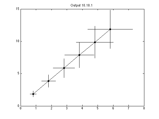
% Problem 10.18.1
%
% The previous chapter introduced the errorbar function to plot a
% vertical line relative to points to show the variability of the
% numbers corresponding to those points. Sometimes behavioral scientists
% plot one dependent variable against another and both sets of dependent
% variables have some variability. Write a program that lets you show
% variability in x as well as in y, similar to the example below. The
% dummy data used to generate this graph happen to have the property
% that variability in x and variability in y both scale with their
% respective means, but that is just an incidental feature of the
% dummy data.
function Solution_10_18_1
fprintf('\n\n %s\n\n','Output 10.18.1')
figure('Name','Solution_10_18_1')
x = [1:6] + randn;
y = (2:2:12) + randn;
sx = .25*x;
sy = .25*y;
plot(x,y,'k.-','markersize',18)
hold on
for j=1:6
% plot y error
plot( [x(j) x(j)],[y(j)-sy(j) y(j)+sy(j)],'k');
% plot x error
plot( [x(j)-sx(j) x(j)+sx(j)],[y(j) y(j)],'k');
end
box on
title('Output 10.18.1')
end % function Solution_10_18_1
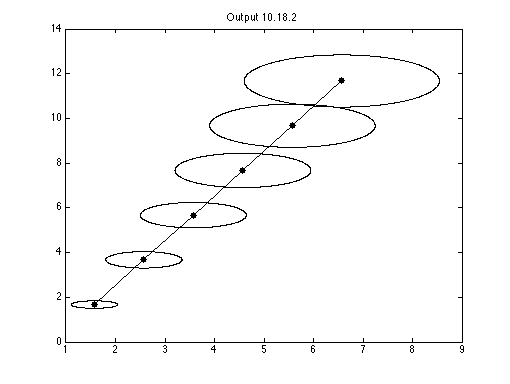
% Problem 10.18.2
%
% Adapt the last program to show ellipses around data points. The
% two axes of the ellipses should correspond to variability along the
% x and y axes, and the output should resemble the graph below. This
% problem may take a little detective work on your part if you don?t
% happen to remember the equation for an ellipse. Consult Wikipedia
% or some other source to find the form of the equation that lends
% itself most easily to MATLAB coding. The fill command was used to
% generate the white ellipses shown below, which are based on the
% same data as in Problem 10.18.1.
%
function Solution_10_18_2
fprintf('\n\n %s\n\n','Output 10.18.2')
figure('Name','Solution_10_18_2')
x = [1:6] + randn;
y = (2:2:12) + randn;
sx = .3 * x;
sy = .1 * y;
hold on
t = linspace(0,2*pi,1000);
for j = 1:length(x)
fill(x(j)+ sx(j)*cos(t),y(j) + sy(j)*sin(t),[1 1 1]);
brighten(.95)
end
plot(x,y,'k.-','markersize',18)
box on
title('Output 10.18.2');
end % function Solution_10_18_2
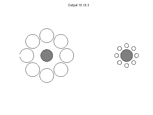
%
% Problem 10.18.3
%
% The Ebbinghaus illusion is a visual illusion in which two circles
% of the same size (the two grey circles below) are seen to be of
% different size depending on the circles around them. Write a program
% to generate images like those below.
%
function Solution_10_18_3
fprintf('\n\n %s\n\n','Output 10.18.3')
figure('Name','Solution_10_18_3')
hold on
t = linspace(0,2*pi,100);
theta = [0:.125:2]*2*pi;
for offset = [-2,2]
if offset == -2
a = .35;
b = 1;
else
a = .1;
b = .5;
end
for i = 1:length(theta)
fill(b*cos(theta(i)) + a*cos(t) + offset,...
b*sin(theta(i)) + a*sin(t),[1 1 1]);
end
a = .3;
%center circle
fill(a*cos(t) + offset, a*sin(t),[.5 .5 .5]);
axis equal
axis off
end
title('Output 10.18.3');
end
% function Solution_10_18_3
%
% Problem 10.18.4
%
% Adapt your 'Ebbinghaus illusion' program so that, from trial to trial,
% circles of constant size are shown in the central position, and
% circles of different sizes and positions are shown around the
% central circles. Write your adapted program so the participant
% can click on whichever central circle seems larger. The participant
% must choose one, so this is an example of a forced choice procedure.
% Determine the range of outer circle sizes and the range of outer circle
% distances from the center of the central circle that lead the
% participant to judge the left central circle as being larger than
% the right central circle between 25% and 75% of the time.
function Solution_10_18_4
fprintf('\n\n %s\n','Output 10.18.4')
fprintf('Solution left to the student.\n\n');
end % function Solution_10_18_4
% Problem 10.18.5
function Solution_10_18_5
fprintf('\n\n %s\n','Output 10.18.5')
fprintf('Solution left to the student.\n\n');
end % function Solution_10_18_5
% Problem 10.18.6
% Use bar3 to visualize the effects of different parameter values on
% one or more statistical distributions of interest to you (or of your
% professor). For example the Weibull distribution relates to failure
% rates over time. It has been applied to such things as the
% characterization of infant mortality rates. Wikipedia or other sources
% can be used to obtain information about statistical distributions.
% For example, Wikipedia includes the following statement in its
% (August 27, 2006) article about the Weibull distribution: "Given a
% random variate U drawn from the uniform distribution in the interval
% (0, 1), then the variate %
% % has a Weibull distribution with parameters k and ?. This follows
% from the form of the cumulative distribution function.? Show the
% effect of and k and ? on X in a 3-dimensional bar graph.
% Problem 10.18.6
%
% Draw on the code in sections 10.9-10.13 to generate one or more
% 3D graphs that show real or simulated data for a behavioral science
% problem of interest to you (or your professor).
function Solution_10_18_6
fprintf('\n\n %s\n','Output 10.18.6')
fprintf('Solution left to the student.\n\n');
end % function Solution_10_18_6
% Problem 10.18.7
%
% Draw on the code in section 10.15 to depict a staircase. Add a railing.
function Solution_10_18_7
fprintf('\n\n %s\n','Output 10.18.7')
fprintf('Solution left to the student.\n\n');
end % function Solution_10_18_7
% Problem 10.18.8
%
% Draw on the code in section 10.17 to show a humanoid descending
% the staircase, or in some other pose that might be useful to you in
% your research.
function Solution_10_18_8
fprintf('\n\n %s\n','Output 10.18.8')
fprintf('Solution left to the student.\n\n');
end % function Solution_10_18_8
% Problem 10.18.9
%
% Repeat the demonstration of Section 10.4, but change the proportion
% of pixels that are white and black. How does that affect the appearance
% of the squares? Add multiple internal squares at different apparent
% depths and/or vary the contrast between the pixels by modifying the
% contents of the color map.
function Solution_10_18_9
fprintf('\n\n %s\n','Output 10.18.9')
fprintf('Solution left to the student.\n\n');
end % function Solution_10_18_9
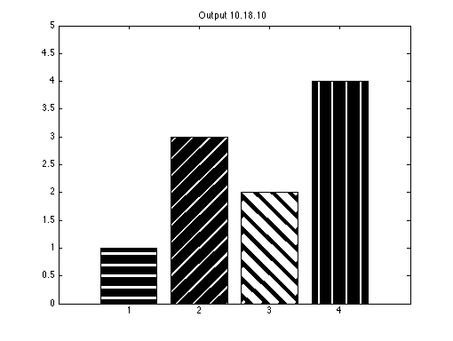
% Problem 10.18.10
%
% MATLAB does not have a good way to make patterned bar graphs that
% show up well in greyscale print. Using what you know about lines,
% explore how to superimpose a pattern of diagonal lines on one of the
% bars in such graph.
function Solution_10_18_10
fprintf('\n\n %s\n\n','Output 10.18.10')
figure('Name','Solution_10_18_10')
data = [1 3 2 4];
bar(data,'k');
leftsides = [1:4] - .4;
rightsides = [1:4] + .4;
for y = 0+.1:.2:data(1)
line([leftsides(1),rightsides(1)],[y,y],'linewidth',3,'color','w');
end
rectangle('position',[leftsides(1),0,.8,data(1)],'EdgeColor','k')
for y = -1:.3:data(2)
line([leftsides(2),rightsides(2)],[y,y+1],'linewidth',2,'color','w');
end
rectangle('position',[leftsides(2),0,.8,data(2)],'edgeColor','k')
for y = 0:.3:data(3)+1
line([leftsides(3),rightsides(3)],[y,y-1],'linewidth',9,'color','w');
end
rectangle('position',[leftsides(3),0,.8,data(3)],'EdgeColor','k')
axis([0,5,0,5])
for x = leftsides(4)+.1:.2:rightsides(4)
line([x,x],[0,data(4)],'linewidth',2,'color','w');
end
rectangle('position',[leftsides(4),0,.8,data(4)],'edgeColor','k')
title('Output 10.18.10');
end % function Solution_10_18_10
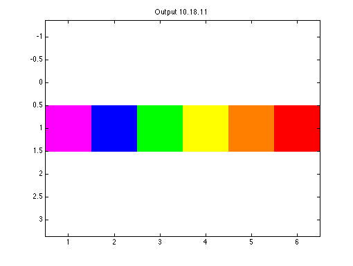
% Problem 10.18.11
%
% Generate the rainbow of output 10.4.1 using a 1×6 image array and
% a 6×3 color map that defines the colors for each of the 6 cells.
function Solution_10_18_11
fprintf('\n\n %s\n\n','Output 10.18.11')
figure('Name','Solution_10_18_11')
clf;
clear;
colors = [
1 0 0 % Red
1 .5 0 % Orange
1 1 0 % Yellow
0 1 0 % Green
0 0 1 % Blue
1 0 1 % Violet
];
rainbow = (1:6);
colormap(colors)
% change the colors of the squares without changing the colormap:
for count = 1:3
rainbow = rainbow(randperm(6));
pause(.5);
image(rainbow)
axis equal
end
title('Output 10.18.11')
end
% ========== Command Window Output follows ==========
Output 10.18.1:
Output 10.18.2:
Output 10.18.3:
Output 10.18.4:
Solution left to the student.
Output 10.18.5:
Solution left to the student.
Output 10.18.6:
Solution left to the student.
Output 10.18.7:
Solution left to the student.
Output 10.18.8:
Solution left to the student.
Output 10.18.9:
Solution left to the student.
Output 10.18.10:
Output 10.18.11: