Code and Output
Code 9.1.1:
% Code_9_1_1.m
clear all
close all
figure(1)
theta_rad = linspace(0,4*(2*pi),100);
plot(theta_rad,sin(theta_rad));
shg
Output 9.1.1:

Code 9.2.1:
% code_9_2_1.m
figure(2)
y = sin(theta_rad);
plot(theta_rad,y);
axis([min(theta_rad) max(theta_rad) min(y) max(y)]);
shg
Output 9.2.1:

Code 9.2.2:
% code_9_2_2.m
figure(3)
x = theta_rad;
plot(x,y);
x_offset = 1;
y_offset = .2;
xlim([min(x)-x_offset, max(x+x_offset)]);
ylim([min(y)-y_offset, max(y+y_offset)]);
shg
Output 9.2.2:

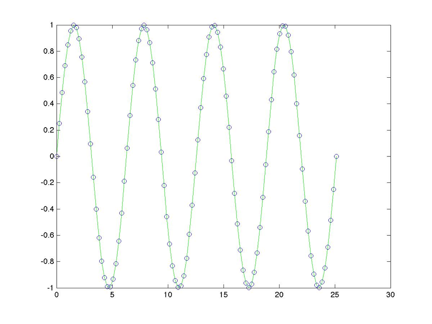
Code 9.3.1:
% code_9_3_1
figure(4);
plot(x,y,'g-');
hold on;
plot(x,y,'bo');
shg;
Output 9.3.1:
Code 9.4.1:
% code_9_4_1.m
figure(5)
theta_rad = 0:.1:2*pi;
y = sin(theta_rad);
plot(theta_rad,y,'go-');hold on;
y = cos(theta_rad);
plot(theta_rad,y,'b-s');
Output 9.4.1:

Code 9.4.2:
help plot
Output 9.4.2:
Various line types, plot symbols and colors may be obtained with PLOT(X,Y,S) where S is a character string made from one element from any or all the following 3 columns:

b     blue     .   point              -     solid
g     green    o   circle             :     dotted
r     red      x   x-mark             -.    dashdot
c     cyan     +   plus               --    dashed
m     magenta  *   star              (none)  no line
y     yellow   s   square
k     black    d   diamond
               v   triangle (down)
               ^   triangle (up)
               <   triangle (left)
               >   triangle (right)
               p   pentagram
               h   hexagram

For example, PLOT(X,Y,'c+:') plots a cyan dotted line with a plus at each data point; PLOT(X,Y,'bd') plots blue diamond at each data point but does not draw any line.
Code 9.4.3:
figure(6)
theta = 0:.1:2*pi;
plot(theta,sin(theta),'c+:',theta,cos(theta),'rd');
shg
Output 9.4.3:

Code 9.5.1:
figure(7)
x = 0:.1:2*pi;
plot(x,sin(x),'ro-','markersize',12);
xlim([min(x)-x_offset, max(x+x_offset)]);
ylim([min(y)-y_offset, max(y+y_offset)]);
box on
shg
Output 9.5.1:

Code 9.5.2:
figure(8)
x = 0:.1:2*pi;
h = plot(cos(x),sin(x), 'r.','markersize',12);
axis equal
get(h)
Output 9.5.2:

h =
DisplayName: ''
 Annotation: [1x1 hg.Annotation]
      Color: [1 0 0]
  LineStyle: 'none'
  LineWidth: 0.5000
     Marker: '.'
 MarkerSize: 12
MarkerEdgeColor: 'auto'
MarkerFaceColor: 'none'
      XData: [1x63 double]
      YData: [1x63 double]
      ZData: [1x0 double]
BeingDeleted: 'off'
ButtonDownFcn: []
   Children: [0x1 double]
   Clipping: 'on'
  CreateFcn: []
  DeleteFcn: []
 BusyAction: 'queue'
HandleVisibility: 'on'
    HitTest: 'on'
Interruptible: 'on'
   Selected: 'off'
SelectionHighlight: 'on'
        Tag: ''
       Type: 'line'
UIContextMenu: []
   UserData: []
    Visible: 'on'
     Parent: 173.0519
  XDataMode: 'manual'
XDataSource: ''
YDataSource: ''
ZDataSource: ''
Code 9.5.3:
figure(9)
x = theta_rad;
plot(x,y,'g-');
hold on
x_offset = 0;
y_offset = .2;
axis([min(x)-x_offset, max(x)+x_offset, ...
      min(y)-y_offset, max(y+y_offset)]);
plot(x,y,'o', 'color,'r','markersize',6,...
    'markeredgecolor','k','markerfacecolor','r');
Output 9.5.3:

Code 9.6.1:
figure(10)
plot(x,y,'g-');
hold on
x_offset = 0;
y_offset = .2;
axis([min(x)-x_offset, max(x)+x_offset, ...
      min(y)-y_offset, max(y+y_offset)]);
plot(x,y,'o','color','r','markersize',6,...
    'markeredgecolor','k','markerfacecolor','r');
xlabel('Time');
ylabel('Happiness');
title('Life has its ups and downs');
Output 9.6.1:

Code 9.7.1:
figure(11)
max_learn = [10 11 12 13];
trial = [1:10];
c1 = max_learn(1) - exp(-trial);
c2 = max_learn(2) - exp(-trial);
c3 = max_learn(3) - exp(-trial);
c4 = max_learn(4) - exp(-trial);

hold on
plot(trial,c4,'g-^');
plot(trial,c3,'m--<');
plot(trial,c2,'b-.>');
plot(trial,c1,'k:v');
legend('Group 4','Group 3',...
       'Group 2','Group 1',...
       'Location','EastOutside');
Output 9.7.1:

Code 9.8.1:
figure(12)
a = 1;           % starting value
b = .5;          % rate parameter
xx = [0:20];
vert_offset = .05;
hor_offset = .50;

y_power = a * xx.^-b;
y_exp = a * exp(b*-xx);

hold on
box on
plot(y_power,'mo-');
plot(y_exp,'kd-');

hor_p = xx(5) + hor_offset;
vert_p = y_power(5) + vert_offset;
text(hor_p,vert_p,'Power function');

hor_e = xx(6) + hor_offset;
vert_e = y_exp(6) + vert_offset;
text(hor_e,vert_e,'Exponential function');
Output 9.8.1:

Code 9.8.2:
clear
close all;
figure('Name','Stroop Test')
words = {
    'Red'
    'Green'
    'Blue'
    'Black'
    };
colors = ['rgbk'];
shg
text(.1,.8,sprintf(...
    'Report the COLOR of the text\n as quickly as you can!'),...
    'FontSize',18)
axis off
for t = 1:20
    w = randi(4);
    c = randi(4);
    myWordHandle = text(.2,.5,...
        char(words(w)),'Color',colors(c),...
        'Fontsize',48);
    if w == c
        conditionstring = sprintf('Compatible trial');
    else
        conditionstring = sprintf('Incompatible trial');
    end
    myConditionHandle = text(.2,.2,conditionstring);
    pause(2)
    delete([myWordHandle myConditionHandle])
    pause(1)
end
Output 9.8.2:

Code 9.9.1:
clear x y
a3 = 0;
a2 = 1;
a1 = 1;
a0 = 0;
x = [-20:20];
randn_coeff = 60;

y = a3*x.^3  + a2*x.^2 + a1*x.^1 + a0*x.^0;
r = rand(length(y))*randn_coeff;
r = r(1,:);
y = y + r;

fitted_coefficients = polyfit(x,y,1);
y_hat1 = fitted_coefficients(1)*x.^1 + ...
    fitted_coefficients(2)*x.^0; %apply polyfit coefficients to x
figure (13)
hold on
plot(y,'bo');         % show original data
plot(y_hat1,'r-');    % show fitted points joined by a line
xlim([0 length(x)]);
box on                % put a box around the graph
c = corrcoef(y, y_hat1);
message = ['Straight line fit: r^2 = ',num2str(c(1,2)^2,3)];
title(message);
Output 9.9.1:

Code 9.9.2:
fitted_coefficients = polyfit(x,y,2);
y_hat2 = fitted_coefficients(1)*x.^2 + ...
         fitted_coefficients(2)*x.^1 + ...
         fitted_coefficients(3)*x.^0;

figure (14)
hold on
plot(y,'bo');         % show original data
plot(y_hat2,'r-');    % show fitted points joined by a line
xlim([0 length(x)]);
box on                % put a box around the graph
c = corrcoef(y, y_hat2);
message = ['Quadratic fit: r^2 = ',num2str(c(1,2)^2,3)];
title(message);
Output 9.9.2:

Code 9.10.1:
figure(15)
x = linspace(0,8*pi,100);

subplot(4,1,1)
plot(cos(x),'r.','markersize',12);
grid on

subplot(4,1,2)
plot(cos(x),'r.','markersize',12);
box on

subplot(4,1,3)
plot(cos(x),'r.','markersize',12);
axis off

subplot(4,1,4)
plot(cos(x),'r.','markersize',12);
axis square
Output 9.10.1:

Code 9.10.2:
figure(15)
clf;

subplot(1,2,1)
plot(cos(x),'r.','markersize',12);
grid on

subplot(1,2,2 )
plot(cos(x),'r.','markersize',12);
grid on
labelhandle = xlabel('Time(secs)')
Output 9.10.2:

Code 9.10.3:
labelposition = get(labelhandle,'Position')
labelposition(1) = labelposition(1) - 65;
labelposition(2) = labelposition(2) + .05;
labelposition
set(labelhandle,'Position',labelposition,'Fontsize',18);
Output 9.10.3:

Output 9.10.4:
labelposition =
49.7312   -1.1316    1.0001
labelposition =
-15.2688   -1.0816    1.0001
Code 9.11.1:
function main
figure(16);
clf
clear x y
x = [1:10];
y = x + 1;
subplot(4,2,1:2);   % In the 4 rows and 2 columns of subplots,
                    % subplots 1 and 2
xlim([0 1]);
ylim([0 1]);
axis off
text(-.05,.05,'                          A Banner Year',...
    'fontsize',24);
subplot(4,2,3);     % In the 4 rows and 2 columns of subplots,
                    % subplot 3
plot(x,y,'k')
text_in_box(.05,.80,'A')
subplot(4,2,4);     % In the 4 rows and 2 columns of subplots,
                    % subplot 4
plot(x,y,'k')
text_in_box(.05,.80,'B')
subplot(4,2,[5 7]); % In the 4 rows and 2 columns of subplots,
                    % subplots 5 and 7
plot(x,y,'k')
text_in_box(.05,.90,'C')
subplot(4,2,6);     % In the 4 rows and 2 columns of subplots,
                    % subplot 6
plot(x,y,'k')
text_in_box(.05,.80,'D')
subplot(4,2,8);     % In the 4 rows and 2 columns of subplots,
                    % subplot 8
plot(x,y,'k')
text_in_box(.05,.80,'E')
Code 9.11.2:
function text_in_box(x_place,y_place,s)

xs = xlim;
ys = ylim;
text(x_place*xs(2),y_place*ys(2),s);
Output 9.11.1:

Code 9.12.1:
get(gca)
Output 9.12.1:
  ActivePositionProperty = position
ALim = [0 1]
ALimMode = auto
AmbientLightColor = [1 1 1]
Box = on
CameraPosition = [5 7.5 17.3205]
CameraPositionMode = auto
CameraTarget = [5 7.5 0]
CameraTargetMode = auto
CameraUpVector = [0 1 0]
CameraUpVectorMode = auto
CameraViewAngle = [6.60861]
CameraViewAngleMode = auto
CLim = [0 1]
CLimMode = auto
Color = [1 1 1]
CurrentPoint = [ (2 by 3) double array]
ColorOrder = [ (7 by 3) double array]
DataAspectRatio = [5 7.5 1]
DataAspectRatioMode = auto
DrawMode = normal
FontAngle = normal
FontName = Helvetica
FontSize = [10]
FontUnits = points
FontWeight = normal
GridLineStyle = :
Layer = bottom
LineStyleOrder = -
LineWidth = [0.5]
MinorGridLineStyle = :
NextPlot = replace
OuterPosition = [0.534263 0.0790476 0.409654 0.20298]
PlotBoxAspectRatio = [1 1 1]
PlotBoxAspectRatioMode = auto
Projection = orthographic
Position = [0.570341 0.11 0.334659 0.157742]
TickLength = [0.01 0.025]
TickDir = in
TickDirMode = auto
TightInset = [0.0285714 0.0309524 0.0142857 0.0142857]
Title = [397.002]
Units = normalized
View = [0 90]
XColor = [0 0 0]
XDir = normal
XGrid = off
XLabel = [394.002]
XAxisLocation = bottom
XLim = [0 10]
XLimMode = auto
XMinorGrid = off
XMinorTick = off
XScale = linear
XTick = [0 5 10]
XTickLabel =
     0
     5
     10
XTickLabelMode = auto
XTickMode = auto
YColor = [0 0 0]
YDir = normal
YGrid = off
YLabel = [395.002]
YAxisLocation = left
YLim = [0 15]
YLimMode = auto
YMinorGrid = off
YMinorTick = off
YScale = linear
YTick = [0 5 10 15]
YTickLabel =
     0
     5
     10
     15
YTickLabelMode = auto
YTickMode = auto
ZColor = [0 0 0]
ZDir = normal
ZGrid = off
ZLabel = [396.002]
ZLim = [-1 1]
ZLimMode = auto
ZMinorGrid = off
ZMinorTick = off
ZScale = linear
ZTick = [-1 0 1]
ZTickLabel =
ZTickLabelMode = auto
ZTickMode = auto

BeingDeleted = off
ButtonDownFcn =
Children = [ (2 by 1) double array]
Clipping = on
CreateFcn =
DeleteFcn =
BusyAction = queue
HandleVisibility = on
HitTest = on
Interruptible = on
Parent = [16]
Selected = off
SelectionHighlight = on
Tag =
Type = axes
UIContextMenu = []
UserData = []
Visible = on
Code 9.12.2:
figure(17)
x = linspace(0,4*(2*pi),100);
y = sin(x);
plot(x,y);
plot(x,y,'g-');
hold on
x_offset = 0;
y_offset = .2;
axis([min(x)-x_offset, max(x)+x_offset, ...
    min(y)-y_offset, max(y+y_offset)]);
plot(x,y,'o','color','r','markersize',6,...
    'markeredgecolor','k','markerfacecolor','r');
xlabel('Time');
ylabel('Happiness');
title('Life has its ups and downs.');
set(gca,'xtick',[2:2:24]);
Output 9.12.2:

Code 9.12.3:
figure(18)
plot(x,y,'g-');
hold on
x_offset = 0;
y_offset = .2;
axis([min(x)-x_offset, max(x)+x_offset, ...
      min(y)-y_offset, max(y+y_offset)]);
plot(x,y,'o','color','r','markersize',6,...
    'markeredgecolor','k','markerfacecolor','r');
xlabel('Time');
ylabel('Happiness');
title('Life has its ups and downs.');
set(gca,'xtick',[]);
set(gca,'ytick',[]);
Output 9.12.3:

Code 9.13.1:
figure(19)
x= [1:10];
y1 = [4 11 25 65 141 191 313 301 487 673];
sd = [20 30 40 50 58 69 82 78 42 62];
box on
hold on
errorbar(x,y1,sd,'ko-','markersize',6)
hold on
y2 = 700-y1;
sdup = sd;
sddown = zeros(length(sdup),1);
errorbar(x,y2,sddown,sdup,'k.','markersize',18)
shg
Output 9.13.1:

Code 9.14.1:
originalradiuspoints = [1 0];
radiusrotated30deg_from_original = [.866 .5];
radiusrotated150deg_from_original = [ -.866 .5];
h1 = compass(originalradiuspoints(1),...
             originalradiuspoints(2));
hold on;
set(h1,'linestyle','-','linewidth',3);

h2 = compass(radiusrotated30deg_from_original(1),...
             radiusrotated30deg_from_original(2));
set(h2,'linestyle','--','linewidth',3);

h3 = compass(radiusrotated150deg_from_original(1),...
             radiusrotated150deg_from_original(2));
set(h3,'linestyle',':','linewidth',3);
Output 9.14.1:

Code 9.15.1:
figure(21)
rng('default')
sample = randn(1,2000) + 5;
[N,X] = hist(sample,[2:8])
hist(sample,[2:8])
colormap([.5 .5 .5])
brighten(.75)
Output 9.15.1:

Output 9.15.2:
N =
6   125   473   788   476   108    24
X =
2     3     4     5     6     7     8
Code 9.16.1:
figure(22)
a = [3 4 5 6 7 6 5 4 3];
barh(a)
colormap([.5 .5 .5])  % gray bars
%  colormap([0 0 0]   % black bars
%  colormap([1 1 1])  % white bars
%  colormap([1 0 0])  % red bars
%  colormap([0 1 0])  % green bars
%  colormap([0 0 1])  % blue bars
brighten(.15)
ylim([0 ,10])
xlim([0 8])
Output 9.16.1:

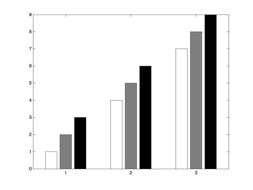
Code 9.16.2:
close all;
clear all;
figure(22)
data = [
1 2 3
4 5 6
7 8 9];
bar(data);
colors = [
    1 1 1
    .5 .5  .5
    0 0 0];
colormap(colors)
Output 9.16.2:
Code 9.17.1:
figure(23)
plot([1:10],[1:10].^-2,'k-o')
print -r600 -djpeg Output_9_17_1

figure(24)
plot([1:10],[1:10].^-2,'k-s')
print -dtiff Output_9_17_2

figure(25)
plot([1:10],[1:10].^-2,'k-^')
print -deps -loose  Output_9_17_3
Output 9.17.1:

Output 9.17.2:

Output 9.17.3:

Code 9.18.1:
set(gcf, 'Position', [100 200 500 500])
Code 9.19.1:
figure(1)
x = linspace(0,1,200);
a = 6;
b = 6;
y = (x.^a).*((1-x).^b);
plot(x,y,'k')
Output 9.19.1:
Solutions
% Solutions_Chapter_09
% Solutions for selected problems from MATLAB for Behavioral Scientists,
% Second Edition (D. A. Rosenbaum, J. Vaughan, & B. Wyble),
% (c) 2015, Taylor & Francis
% To generate the solution for one problem, copy and run the code for that
% problem in a file or paste it into the Command window. Show the Command
% window to see the results.
% To generate sll the solutions for Chapter 9, save this code as a
% MATLAB script file and run the program.
function main % Problems in this chapter will have nested or local
% functions so the Solutions file must itself be a function
close all
clc
commandwindow
Solution_9_19_1 %Run each of the problem functions in turn.
Solution_9_19_2
Solution_9_19_3
Solution_9_19_4
Solution_9_19_5
Solution_9_19_6
shg
fprintf('\n\n ========== Graphic Output follows ==========\n\n');
end % function main
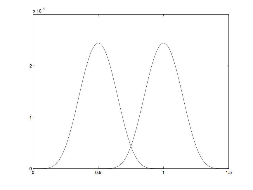
% Problem 9.19.1
% The following code will yield one bell-shaped curve. Modify the code
% to get two bell-shaped curves, with one shifted .5 units to the right
% of the other, as shown in the figure after the code below.
% figure(1)
% x = linspace(0,1,200);
% a = 6;
% b = 6;
% y = (x.^a).*((1-x).^b);
% plot(x,y,'k')
function Solution_9_19_1
fprintf('\n\n %s\n\n','Output 9.19.1')
figure('Name','Solution_9_19_1')
x = linspace(0,1,200);
a = 6;
b = 6;
y = (x.^a).*((1-x).^b);
plot(x,y,'k'); hold on;
plot(x+.5,y,'k');
title('Output 9.19.1')
end % function Solution_9_19_1
% Problem 9.19.2
% Problem 5.9.5 referred to the equation
% p_correct = base_rate + learning_rate*log(trial),
% where trial could take on the values 1, 2, 3, ..., 200, learning_rate
% could be any real number between 0 and 1, base_rate was ¼, and
% p_correct could not exceed 1. Generate a figure resembling the
% one below by setting learning_rate to .02. Plot p_correct as a
% function of trial, label the x axis Trials, label the y axis
% Proportion Correct, and have the title say Learning. Have the
% points appear as black o's connected with line segments. The
% grid should be on, the box should be on.
function Solution_9_19_2
fprintf('\n\n %s\n\n','Output 9.19.2')
figure('Name','Solution_9_19_2')
base_rate = .25;
learning_rate = .02;
trial = [1:200];
for i = 1:max(trial)
p_correct(i) = base_rate + learning_rate*log(trial(i));
if p_correct(i) > 1
p_correct(i) = 1;
end
end
plot(p_correct,'bo-')
xlabel('Trials')
ylabel('Proportion Correct')
title('Learning')
grid on
box on
title('Output 9.19.2')
end %function Solution_9_19_2
% Problem 9.19.3
% Adapt the program you wrote for the last problem to generate a
% figure resembling the one below by setting learning_rate to .02,
% .04, and .06.
%
function Solution_9_19_3
fprintf('\n\n %s\n\n','Output 9.19.3')
figure('Name','Solution_9_19_3')
for lr = 1:3
base_rate = .25;
learning_rate(lr) = .02*lr;
trial = [1:200];
for i = 1:max(trial)
p_correct(i) = base_rate + ...
learning_rate(lr)*log(trial(i));
if p_correct(i) > 1
p_correct(i) = 1;
end
end
plot(p_correct,'ko-')
xlabel('Trials')
ylabel('Proportion Correct')
title('Learning')
grid on
box on
hold on
end
title('Output 9.19.3')
end % function Solution_9_19_3
% Problem 9.19.4
%
% Adapt the program you wrote for the last problem to generate a
% figure resembling the one below by again setting learning_rate to
% .02, .04, and .06 and making the subplots on the right show the
% cumulative number correct for each of the three learning
% rates.
%
function Solution_9_19_4
fprintf('\n\n %s\n\n','Output 9.19.4')
figure('Name','Solution_9_19_4')
for lr = 1:3
cump(1)= 0;
base_rate = .25;
learning_rate(lr) = .02*lr;
trial = [1:200];
for i = 1:max(trial)
p_correct(i) = base_rate + ...
learning_rate(lr)*log(trial(i));
if p_correct(i) > 1
p_correct(i) = 1;
end
if i > 1
cump(i) = cump(i-1) + p_correct(i);
end
end
subplot(3,2,(lr*2)-1)
plot(p_correct,'ko-')
ylim([0 .6])
xlabel('Trials')
ylabel('Proportion Correct')
if (lr) == 1
title('Output 9.19.4')
end;
subplot(3,2,lr*2)
plot(cump,'k')
hold on
ylim([0 100])
xlabel('Trials')
ylabel('Total Correct')
grid on
box on
hold on
end
end % function Solution_9_19_4
% Problem 9.19.5
%
% Adapt the program you wrote for the last problem to generate a
% figure that resembles the one below. There are two new features
% of the figure to be generated. One is that the learning rates are
% specified as text in each of the left subplots. The other is that
% the subplots on the right include a star at the trial for which
% the cumulative number correct exceeds 50.
%
function Solution_9_19_5
fprintf('\n\n %s\n\n','Output 9.19.5')
figure('Name','Solution_9_19_5')
for lr = 1:3
cump(1)= 0;
special_i = NaN;
special_cump = NaN;
base_rate = .25;
learning_rate(lr) = .02*lr;
trial = [1:200];
for i = 1:max(trial)
p_correct(i) = base_rate + ...
learning_rate(lr)*log(trial(i));
if p_correct(i) > 1
p_correct(i) = 1;
end
if i > 1
cump(i) = cump(i-1) + p_correct(i);
end
end
if any(cump>50)
cumpGT50 = find(cump > 50);
special_i = cumpGT50(1);
special_cump = cump(special_i);
end
subplot(3,2,(lr*2)-1)
plot(p_correct,'ko-')
ylim([0 .6])
text(40,.2,['Learning rate = ' ...
num2str(learning_rate(lr))]);
if (lr) == 1
title('Output 9.19.5')
end;
xlabel('Trials')
ylabel('Proportion Correct')
subplot(3,2,lr*2)
plot(cump,'k')
hold on
if special_cump ~= nan
plot(special_i,special_cump,'k*','markersize',22)
end
ylim([0 100])
xlabel('Trials')
ylabel('Total Correct')
grid on
box on
hold on
end
title('Output 9.19.5')
end % function Solution_9_19_5
% Problem 9.19.6
% Given these made-up data:
%
% Lefthanders:
% Condition RT (ms)
% Valid
% Left 240
% Right 230
% Invalid
% Left 270
% Right 260
% Righthanders:
% Condition RT (ms)
% Valid
% Left 210
% Right 220
% Invalid
% Left 280
% Right 290
%
% Plot the data in two adjacent 2x2 subplots with appropriately
% labeled axes. Try bar graph and line graph styles. Make nice big
% points. By inspection, does there seem to be a statistical interaction
% in this hypothetical experiment?
% Which kind of graph shows that the best?
function Solution_9_19_6
fprintf('\n\n %s\n\n','Output 9.19.6')
data.LH.V.left = 240;
data.LH.V.right = 230;
data.LH.I.left = 270;
data.LH.I.right = 260;
data.RH.V.left = 210;
data.RH.V.right = 220;
data.RH.I.left = 280;
data.RH.I.right = 290;
figure('Name','Solution_9_19_6')
subplot(2,2,1);
bar([data.LH.V.left data.LH.I.left;data.LH.V.right data.LH.I.right]);
axis([0 3 200 300])
set(gca,'XTick',[1 2])
set(gca,'XTickLabel',{'left' 'right'});
set(gca,'Fontsize',14);
legend('Valid','Invalid');
title('LeftHanders','FontSize',16,'FontWeight','bold')
subplot(2,2,2)
hold on;
bar([data.RH.V.left data.RH.I.left;data.RH.V.right data.RH.I.right]);
axis([0 3 200 300])
set(gca,'XTick',[1 2])
set(gca,'XTickLabel',{'left' 'right'});
set(gca,'Fontsize',14);
title('RightHanders','FontSize',16,'FontWeight','bold')
box on;
subplot(2,2,3);
plot([data.LH.V.left data.LH.V.right],'-ob','Linewidth',2);hold on;
plot([data.LH.I.left data.LH.I.right],'-or','Linewidth',2);
axis([0 3 200 300])
set(gca,'XTick',[1 2])
set(gca,'XTickLabel',{'left' 'right'});
set(gca,'Fontsize',14);
hx = xlabel('Stimulus side','FontSize',16,'FontWeight','bold');
set(hx,'Position', get(hx,'Position') + [2 0 0]);
hy = ylabel('Reaction time (ms)','FontSize',16,'FontWeight','bold');
set(hy,'Position', get(hy,'Position') + [0 75 0]);
box on;
subplot(2,2,4)
hold on;
plot([data.RH.V.left data.LH.V.right],'-ob','Linewidth',2);hold on;
plot([data.RH.I.left data.RH.I.right],'-or','Linewidth',2);
axis([0 3 200 300])
set(gca,'XTick',[1 2])
set(gca,'XTickLabel',{'left' 'right'});
set(gca,'Fontsize',14);
thandle = title('Output 9.19.6');
tpos = get(thandle,'Position');
set(thandle,'Position',tpos + [-2 143 0]);
box on;
end % function Solution_9_19_6
Output 9.19.1:

Output 9.19.2:

Output 9.19.3:

Output 9.19.4:

Output 9.19.5:

Output 9.19.6:
